Rolling Regression
Rolling regressions are one of the simplest models for analysing changing relationships among variables overtime. They use linear regression but allow the data set used to change over time. In most linear regression models, parameters are assumed to be time-invariant and thus should not change overtime. Rolling regressions estimate model parameters using a fixed window of time over the entire data set. A larger sample size, or window, used will result in fewer parameter estimates but use more observations. For more information, see Base on Rolling.
Keep in Mind
- When setting the width of your rolling regression you are also creating the starting position of your analysis given that it needs the a window sized amount of data begin.
Also Consider
- An expanding window can be used where instead of a constantly changing fixed window, the regression starts with a predetermined time and then continually adds in other observations until the entire data set is used.
Implementation
Python
This example will make use of the statsmodels package, and some of the description of rolling regression has benefitted from the documentation of that package.
Rolling ordinary least squares applies OLS (ordinary least squares)
across a fixed window of observations and then rolls (moves or slides)
that window across the data set. The key parameter is window, which
determines the number of observations used in each OLS regression.
First, let’s import the packages we’ll be using. If you don’t already
have these installed, open up your terminal (aka command line) and use
the command pip install packagename where ‘packagename’ is the package
you want to install.
from statsmodels.regression.rolling import RollingOLS
import statsmodels.api as sm
from sklearn.datasets import make_regression
import matplotlib.pyplot as plt
import pandas as pd
Next we’ll create some random numbers to do our regression on
X, y = make_regression(n_samples=200, n_features=2, random_state=0, noise=4.0,
                       bias=0)
df = pd.DataFrame(X).rename(columns={0: 'feature0', 1: 'feature1'})
df['target'] = y
df.head()
| feature0 | feature1 | target | |
|---|---|---|---|
| 0 | -0.955945 | -0.345982 | -36.740556 |
| 1 | -1.225436 | 0.844363 | 7.190031 |
| 2 | -0.692050 | 1.536377 | 44.389018 |
| 3 | 0.010500 | 1.785870 | 57.019515 |
| 4 | -0.895467 | 0.386902 | -16.088554 |
Now let’s fit the model using a formula and a window of 25 steps.
roll_reg = RollingOLS.from_formula('target ~ feature0 + feature1 -1', window=25, data=df)
model = roll_reg.fit()
Note that -1 just suppresses the intercept. We can see the parameters
using model.params. Here are the params for time steps 20 to 30:
model.params[20:30]
| feature0 | feature1 | |
|---|---|---|
| 20 | NaN | NaN |
| 21 | NaN | NaN |
| 22 | NaN | NaN |
| 23 | NaN | NaN |
| 24 | 20.736214 | 35.287604 |
| 25 | 20.351719 | 35.173493 |
| 26 | 20.368027 | 35.095621 |
| 27 | 20.532655 | 34.919468 |
| 28 | 20.470171 | 35.365235 |
| 29 | 20.002261 | 35.666997 |
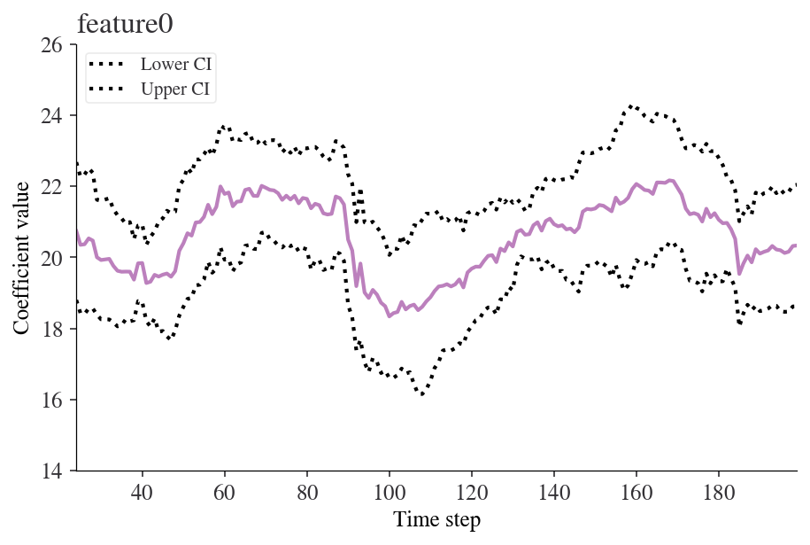
Note that there aren’t parameters for entries between 0 and 23 because our window is 25 steps wide. We can easily look at how any of the coefficients are changing over time. Here’s an example for ‘feature0’.
fig = model.plot_recursive_coefficient(variables=['feature0'])
plt.xlabel('Time step')
plt.ylabel('Coefficient value')
plt.show()
Recursive ordinary least squares (aka expanding window rolling regression)
A rolling regression with an expanding (rather than moving) window
is effectively a recursive least squares model. We can perform this kind
of estimation using the RecursiveLS function from statsmodels.
Let’s fit this to the whole dataset:
reg_rls = sm.RecursiveLS.from_formula(
    'target ~ feature0 + feature1 -1', df)
model_rls = reg_rls.fit()
print(model_rls.summary())
                           Statespace Model Results
==============================================================================
Dep. Variable:                 target   No. Observations:                  200
Model:                    RecursiveLS   Log Likelihood                -570.923
Date:                Sun, 23 May 2021   R-squared:                       0.988
Time:                        17:05:03   AIC                           1145.847
Sample:                             0   BIC                           1152.444
                                - 200   HQIC                          1148.516
Covariance Type:            nonrobust   Scale                           17.413
==============================================================================
                 coef    std err          z      P>|z|      [0.025      0.975]
------------------------------------------------------------------------------
feature0      20.6872      0.296     69.927      0.000      20.107      21.267
feature1      34.0655      0.302    112.870      0.000      33.474      34.657
===================================================================================
Ljung-Box (Q):                       40.19   Jarque-Bera (JB):                 3.93
Prob(Q):                              0.46   Prob(JB):                         0.14
Heteroskedasticity (H):               1.17   Skew:                            -0.31
Prob(H) (two-sided):                  0.51   Kurtosis:                         3.31
===================================================================================

Warnings:
[1] Parameters and covariance matrix estimates are RLS estimates conditional on the entire sample.
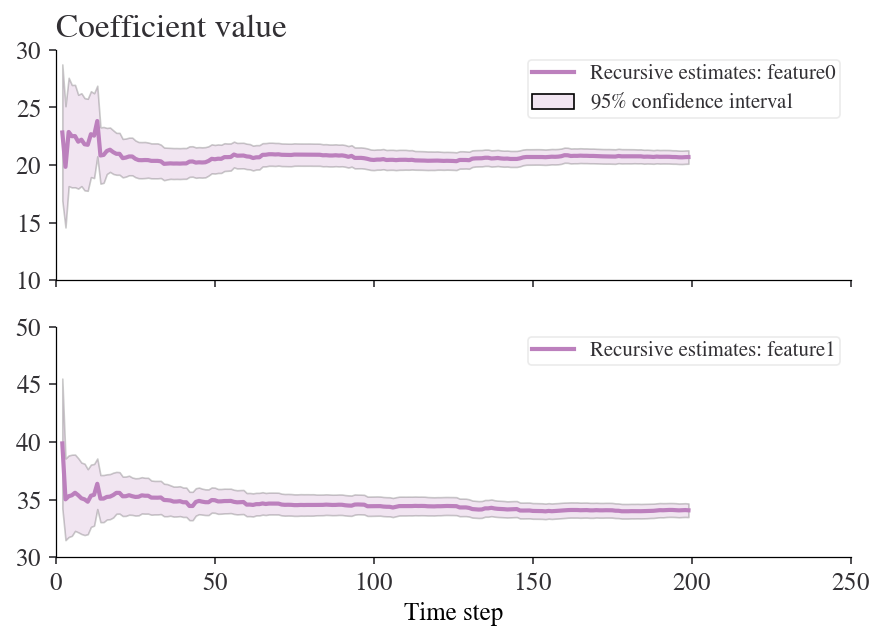
But now we can look back at how the values of the coefficients changed in real time:
fig = model_rls.plot_recursive_coefficient(range(reg_rls.k_exog), legend_loc='upper right')
ax_list = fig.axes
for ax in ax_list:
    ax.set_xlim(0, None)
ax_list[-1].set_xlabel('Time step')
ax_list[0].set_title('Coefficient value');
R
In R the rollRegres (one s, not two) package can compute rolling regressions while being able to specify the linear regression, window size, whether you want a rolling or expanding window, the minimum number of observations required in a window, and other options.
#Load in the package
library(rollRegres)
The data will be manually created where x can be interpreted as any independent variable over a fixed time period, and y is an outcome variable.
#Simulate data
set.seed(29132867)
n <- 200
p <- 2
X <- cbind(1, matrix(rnorm(p * n), ncol = p))
y <- drop(X %*% c(1, -1, 1)) + rnorm(n)
df_1 <- data.frame(y, X[, -1])

#Run the rolling regression (Rolling window)
roll_rolling <- roll_regres(y ~ X1, df_1, width = 25L, do_downdates = TRUE)

#Check the first 10 coefficients
roll_rolling$coefs %>% tail(25)
##     (Intercept)         X1
## 176    1.467609 -1.1887381
## 177    1.561271 -1.0356878
## 178    1.598559 -1.0142755
## 179    1.615713 -0.8161185
## 180    1.680253 -0.8814448
## 181    1.593962 -0.8878947
## 182    1.623287 -1.0246186
## 183    1.596735 -1.0535530
## 184    1.761971 -0.9466231
## 185    1.703679 -0.8138562
## 186    1.619849 -0.8948204
## 187    1.729696 -0.9266218
## 188    1.606376 -1.0624713
## 189    1.676579 -0.9823355
## 190    1.657288 -1.0377997
## 191    1.579115 -1.1432474
## 192    1.586334 -1.1829136
## 193    1.393517 -1.1447650
## 194    1.250160 -1.0244144
## 195    1.243020 -1.0232251
## 196    1.205068 -1.0201693
## 197    1.273287 -0.9792404
## 198    1.336927 -0.9346933
## 199    1.343452 -0.9316855
## 200    1.284072 -0.9379035
To demonstrate the point about a starting position for your analysis, the entries up to 24 are null because of the choice of window size.
#Check the first 25 coefficients
roll_rolling$coefs %>% head(25)
##    (Intercept)        X1
## 1           NA        NA
## 2           NA        NA
## 3           NA        NA
## 4           NA        NA
## 5           NA        NA
## 6           NA        NA
## 7           NA        NA
## 8           NA        NA
## 9           NA        NA
## 10          NA        NA
## 11          NA        NA
## 12          NA        NA
## 13          NA        NA
## 14          NA        NA
## 15          NA        NA
## 16          NA        NA
## 17          NA        NA
## 18          NA        NA
## 19          NA        NA
## 20          NA        NA
## 21          NA        NA
## 22          NA        NA
## 23          NA        NA
## 24          NA        NA
## 25    1.401621 -1.127908
Finally, here are the results when using an expanding window (also known as recursive regression)
#Run the rolling regression (Rolling window)
roll_expanding <- roll_regres(y ~ X1, df_1, width = 25L,do_downdates = FALSE)

#Check the last 10 coefficients
roll_expanding$coefs %>% tail(10)
##     (Intercept)        X1
## 191    1.189651 -1.066285
## 192    1.196722 -1.077508
## 193    1.180968 -1.068470
## 194    1.178508 -1.064603
## 195    1.177739 -1.064419
## 196    1.170369 -1.063868
## 197    1.172466 -1.064678
## 198    1.179917 -1.056945
## 199    1.181876 -1.056017
## 200    1.178556 -1.054890