Introduction
Economic theory usually suggests other variables that could help to forecast the variable of interest over than itself. When we add other variables and their lags the result is what is known as The Autoregressive Lag (ADL) Model. For example, if we want to predict future changes in inflation, the theory (Phillips Curve) suggests that lagged values of the unemployment rate might be a good predictor.
In particular, the method for indicating when one variable possibly causes a response in another is called the Granger Causality Test. But be careful and do not get confused with the name. The test does not strictly mean that we have estimated the causal effect of one variable on another. It means that the signal of the first one is a useful predictor of the second.
A variable \(X\) is said to Granger cause another variable \(Y\) if \(Y\) can be better predicted from the past of \(X\) and \(Y\) together than the past of \(Y\) alone, other relevant information being used in the prediction (Pierce, 1977).
Keep in Mind
-
Check that both series are stationary. If necessary, transform the data via logarithms or differences.
-
Estimate the model with lags enough to ensure white noise residuals.
- When you are choosing the number of lags one variable might affect the other, there is a trade-off between bias and power. To see more click here.
-
Re-estimate both models, including the lags of the other variable.
\[Y_t = \alpha + \sum_{j=1}^{p} \beta_j Y_{t-j} + \sum_{j=1}^r \theta_j X_{t-j}+ \epsilon_t\] \[X_t = \alpha^{\ast} + \sum_{j=1}^{p} \beta_j^{\ast} Y_{t-j} + \sum_{j=1}^r \theta_j^{\ast} X_{t-j}+ \epsilon_t^{\ast}\]-
\(X_t\) helps to predict \(Y_t\) if \(\theta_j \neq 0\) for some \(j\).
-
\(Y_t\) helps to predict \(X_t\) if \(\theta_j^{\ast} \neq 0\) for some \(j\).
-
-
Use an F test to determine significance of the new variables. Consider the following ADL model:
\[H_0: \theta_j^{\ast} =0 \quad \text{for all} \quad j = 1,\dots, r \quad \text{by means of F-test}.\]- Interpretation: \(X\) Granger causes \(Y\) if it helps to predict \(Y\), whereas \(Y\) does not help to predict \(X\).
Also consider
- You might also be interested in a Nonparametric Test for Granger Causality. Especially useful to examine a large number of lags, and flexible to find Granger causality in specific regions on the distribution. See more here
Implementation
R
More information about ADL modeling with R is available in Chapter 14 of Hanck et al. (freely available online).
Simulation ADL model
NOTE: Feel free to skip this section if you are just interested in how to apply the test.
# set seed
set.seed(1234)

# Simulate error
n     = 200 # Sample size
rho   = 0.5 # Correlation between Y errors
coe   = 1.2 # Coefficient of X in model Y
alpha = 0.5 # Intercept of the model Y

# Function to create the error of Y
ARsim2 = function(rho, first, serieslength, distribution) {
  if (distribution=="runif") {
     a = runif(serieslength,min=0,max=1)
  } else {
     a = rnorm(serieslength,0,1)
  }
  Y = first
  for (i in (length(rho)+1):serieslength) {
    Y[i] = rho*Y[i-1]+(sqrt(1-(rho^2)))*a[i]
  }
  return(Y)
}

# Error for Y model
error = ARsim2(rho, c(0, 0), n, "rnorm")

# times series X (simulation)
X = arima.sim(list(order = c(1, 0, 0), ar = c(0.2)), n)

# times series Y (simulation)
Y = NULL
for (i in 2:200) {
  Y[i] = alpha + (coe * X[i - 1]) + error[i]
}
Data
data = as.data.frame(cbind(1:200,X,as.ts(Y)))
colnames(data) = c("time", "X","Y")
Graph
# If necessary
# install.packages("tidyr")
# install.packages("ggplot2")

library(tidyr)
library(ggplot2)

graphdata =
  data[2:200,] |>
  pivot_longer(cols = -c(time), names_to="variable", values_to="value")

ggplot(graphdata, aes(x = time, y = value, group=variable)) +
  geom_line(aes(color = variable), size = 0.7) +
  scale_color_manual(values = c("#00AFBB", "#E7B800")) +
  theme_minimal()+
  labs(title = "Simulated ADL models")+
  theme(text = element_text(size = 15))
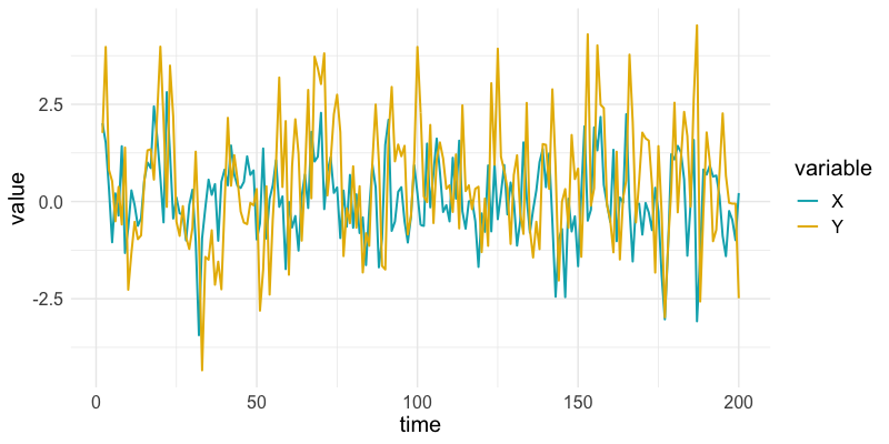
It seems that:
- Both series are stationary (later is check with the ADF test), and
- Disturbances in variable \(X\) are visible after periods in \(Y\) (as expected).
Check Stationarity
# If necessary
# install.packages("tseries")
library(tseries)

## ADF test
adf.test(X, k=3)
adf.test(na.omit(Y), k=3) #na.omit() to delete the first 2 periods of lag
- With a p-value of 0.01 and 0.01 for series \(X\), and \(Y\), we assure that both are stationary.
- No transformation needed for the series.
Granger Test
Note: grangertest() only performs tests for Granger causality in bivariate series.
Step 1. \((Y \sim X)\)
# If neccesary
# install.packages("lmtest")
library(lmtest)
grangertest(Y ~ X, order = 2, data = data)
## Granger causality test
##
## Model 1: Y ~ Lags(Y, 1:2) + Lags(X, 1:2)
## Model 2: Y ~ Lags(Y, 1:2)
##   Res.Df Df      F    Pr(>F)
## 1    192
## 2    194 -2 198.42 < 2.2e-16 ***
## ---
## Signif. codes:  0 '***' 0.001 '**' 0.01 '*' 0.05 '.' 0.1 ' ' 1
Step 2. \((X \sim Y)\)
grangertest(X ~ Y, order = 2, data = data)
## Granger causality test
##
## Model 1: X ~ Lags(X, 1:2) + Lags(Y, 1:2)
## Model 2: X ~ Lags(X, 1:2)
##   Res.Df Df      F Pr(>F)
## 1    192
## 2    194 -2 1.2028 0.3026
-
We see that the effect of lags of number of \(X\) is highly significant, and conclude that \(X\) predicts the future of \(Y\).
-
The null hypothesis is not rejected for the converse relationship. Thus, we conclude that \(X\) Granger causes \(Y\).
Impulse Response Functions
After establishing that \(X\) predicts the future of \(Y\), it is often useful to show exactly how how a shock in \(X\) in the present will impact \(Y\) in the future. Impulse response functions are a great way to visualize the magnitude and duration of this impact on \(Y\).
Vector Autoregression
In order to visualize the impulse response function, we first need to transform the \(X\) and \(Y\) variables through Vector Autoregression (VAR) modeling. In brief, VAR models are a multivariate generalization of scalar autoregressive (AR) models (for more information, see the AR Models page). Through a multivariate auto regression, we can use the autoregressive elements of each variable to visualize the granger causality we tested for earlier.
VAR modeling can be done through the vars package in R.
# If necessary
# install.packages("vars")

library(vars)

# Select only the X and Y columns and save as time series data
data_ts = ts(data[2:3])

# Remove first lagged observation to omit NA values
data_ts = data_ts |> na.omit()

# Save the model as a vector autoregression (VAR)
model = VAR(data_ts, type = "const")
Plotting the IRF
Now that we have created our VAR model, we can plot how a shock to \(X\) will impact \(Y\). To do this we will use the vars::irf() function and the base R plot() function.
# Create the impulse response function
model_IRF = irf(model)

# Plot
plot(model_IRF)
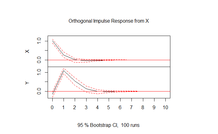
This plot shows the response in \(Y\) to a shock in \(X\). As we would expect from the granger tests we ran earlier, a shock to \(X\) has a statistically significant effect on \(Y\). A positive shock to \(X\) results in a positive shock of similar magnitude in \(Y\) in the following period.
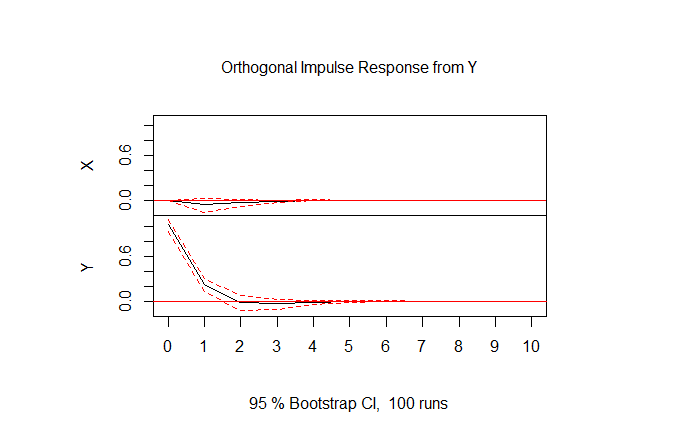
This plot shows the response in \(X\) of a shock to \(Y\). A shock in \(Y\) elicits a very small, not statistically significant effect in \(X\). This is a visual confirmation that \(Y\) does not Granger cause \(X\).
References
Granger, C. W. (1969). Investigating Causal Relations by Econometric Models and Cross-Spectral Methods. Econometrica, 37(3), 424–438.
Pierce, D.A. (1977). $R^2$ Measures for Time Series. Special Studies Paper No. 93, Washington, D.C.: Federal Reserve Board.