Moving Average (MA) Models
Moving Average Models are a common method for modeling linear processes that exhibit serial correlation. This can take many forms, but an easy example is weather patterns.
Imagine we modelled Ski Lift Purchases over a 5 consecutive weekday period. Let weather shocks be identically and independently distributed. A weather shock with large amounts of snow would cause more individuals to go ski. This shock would have future impacts on ski ticket purchases; individuals tomorrow will go skiing due to the snowfall today. This means when we think of the process, we should account for previous shock effects on outcomes today:
\[SkiTicketPurchases_t = \mu + \theta_1*Weather_t + \theta_2*Weather_{t-1}\]Definition
Let \(\epsilon_t \sim N(0, \sigma^2_{\epsilon})\). A moving average process, which is denoted MA(q), take the form as:
\[y_t = \mu + \epsilon_t + \theta_1 \epsilon_{t-1} + ... + \theta_q \epsilon_{t-q}\]Note that a MA(q) process has q lagged \(\epsilon\) terms. Thus a MA(1) process would take the form:
\[y_t = \mu + \epsilon_t + \theta_1 \epsilon_{t-1}\]Properties of a MA(1) process:
- The mean is constant.
- The variance is constant.
- The covariance between \(y_t\) and \(y_{t-q}\) is decreasing as \(q \to \infty\).
Additional helpful information can be found at Wikipedia: Moving Average Models
Keep in Mind
- Time series data needs to be properly formatted (e.g. date columns should be formatted into a time)
- Model Selection uses the Akaike Information Criterion (AIC), Bayesian Information Criterion (BIC), or the Akaike Information Criterion corrected (AICc) to determine the appropriate number of terms to include. Refer to Wikipedia:Model Selection for further information.
Implementations
Julia
MA(q) models in Julia can be estimated using the StateSpaceModels.jl package, which also allows for the estimation of a variety of time series models that have linear state-space representations.
Begin by importing and loading necessary packages into your work environment.
# Load necessary packages
using StateSpaceModels, LinearAlgebra, ShiftedArrays
We may simulate an MA(3) model, where the MA coefficients are set to \(\theta_1 = 0.5\), \(\theta_2 = 0.3\), and \(\theta_3 = 0.2\).
# Set parameters
theta1, theta2, theta3 = (0.5, 0.3, 0.2)

# Draw a sample of an iid N(0,1) disturbance/noise process
# Set number of observations to 1000
u = randn(1000)

# Simulate MA(3) process
 Y = u + theta1 .* lag(u, 1, default = 0.0) + theta2 .* lag(u, 2, default = 0.0) + theta3 .* lag(u, 3, default = 0.0)

# Remove first 3 observations
Y = Y[4:end]
The lag(u, k, default = 0.0) portions of the above code chunk creates a k-lag of series u, and sets the missing observations equal to 0.0.
The data generated by a single sample draw from the above data-generating process can then be assigned a general ARIMA(p,d,q) representation, where if p and d are set to zero, the model specification becomes MA(q). The p=d= 0 constraint can be applied by inputting order = (0,0,q), where q>0.
# Specify the generated Y series as an MA(3) model
model = SARIMA(Y, order = (0,0,3))
Lastly, the above-specified model can be estimated using the fit! function, and the estimation results printed using the results function. The sole input for both of these functions is the model object that contains the chosen data series and its assigned ARIMA structure.
# Fit (estimate) the model
fit!(model)

# Print estimates
results(model)
R
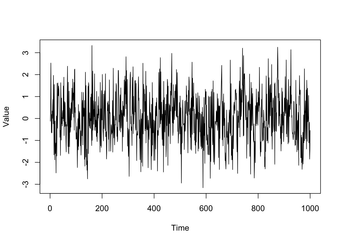
#in the stats package we can simulate an ARIMA Model. ARIMA stands for Auto-Regressive Integrated Moving Average model. We will be setting the AR and I parts to 0 and only simulating a MA(q) model.
set.seed(123)
DT = arima.sim(n = 1000, model = list(ma = c(0.1, 0.3, 0.5)))

plot(DT, ylab = "Value")
set.seed(123)
DT = arima.sim(n = 1000, model = list(ma = c(0.1, 0.3, 0.5)))
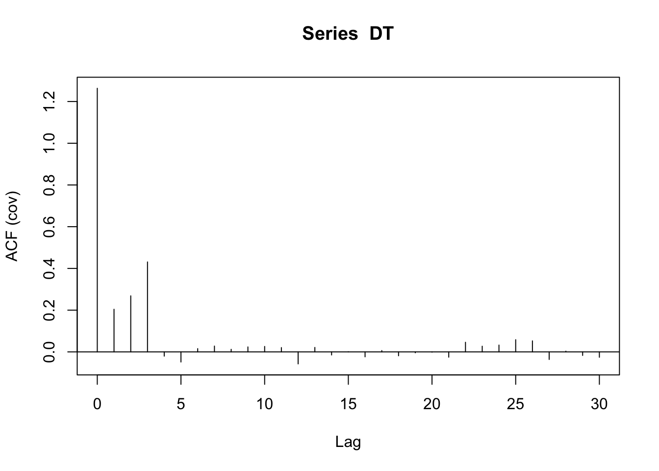
#ACF stands for Autocorrelation Function
#Here we can see that there may be potential for 3 lags in our MA process. (Note: This is due to property (3): the covariance of y_t and y_{t-3} is nonzero while the covariance of y_t and y_{t-4} is 0)
acf(DT, type = "covariance")
set.seed(123)
DT = arima.sim(n = 1000, model = list(ma = c(0.1, 0.3, 0.5)))

#Here I'm estimating an ARIMA(0,0,3) model which is a MA(3) model. Changing c(0,0,q) allows us to estimate a MA(q) process.
arima(x = DT, order = c(0,0,3))

    ##
    ## Call:
    ## arima(x = DT, order = c(0, 0, 3))
    ##
    ## Coefficients:
    ##          ma1     ma2     ma3  intercept
    ##       0.0722  0.2807  0.4781     0.0265
    ## s.e.  0.0278  0.0255  0.0294     0.0573
    ##
    ## sigma^2 estimated as 0.9825:  log likelihood = -1410.63,  aic = 2831.25

#We can also estimate a MA(7) model and see that the ma4, ma5, ma6, and ma7 are close to 0 and insignificant.
arima(x = DT, order = c(0,0,7))


    ##
    ## Call:
    ## arima(x = DT, order = c(0, 0, 7))
    ##
    ## Coefficients:
    ##          ma1     ma2     ma3      ma4      ma5      ma6      ma7  intercept
    ##       0.0714  0.2694  0.4607  -0.0119  -0.0380  -0.0256  -0.0219     0.0267
    ## s.e.  0.0316  0.0321  0.0324   0.0363   0.0339   0.0332   0.0328     0.0533
    ##
    ## sigma^2 estimated as 0.9806:  log likelihood = -1409.65,  aic = 2837.3

#fable is a package designed to estimate ARIMA models. We can use it to estimate our MA(3) model.
library(fable)
#an extension of tidyverse to temporal data (this allows us to create time series data into tibbles which are needed for fable functionality)
library(tsibble)
#visit https://dplyr.tidyverse.org/ to understand dplyr syntax; this package is important for fable functionality
library(dplyr)

#When using the fable package, we need to convert our object into a tsibble (a time series tibble). This gives us a data frame with values and an index for the time periods
DT = DT %>%
  as_tsibble()

head(DT)

    ## # A tsibble: 6 x 2 [1]
    ##   index  value
    ##   <dbl>  <dbl>
    ## 1     1 -0.123
    ## 2     2  0.489
    ## 3     3  2.53
    ## 4     4  0.706
    ## 5     5 -0.640
    ## 6     6  0.182

#Now we can use the dplyr package to pipe our dataset and create a fitted model
#Note: the ARIMA function in the fable package uses an information criterion for model selection; these can be set as shown below; additional information is above in the Keep in Mind section (the default criterion is aicc)
MAfit = DT %>%
  model(arima = ARIMA(value, ic = "aicc"))

#report() is needed to view our model
report(MAfit)

    ## Series: value
    ## Model: ARIMA(0,0,3)
    ##
    ## Coefficients:
    ##          ma1     ma2     ma3
    ##       0.0723  0.2808  0.4782
    ## s.e.  0.0278  0.0255  0.0294
    ##
    ## sigma^2 estimated as 0.9857:  log likelihood=-1410.73
    ## AIC=2829.47   AICc=2829.51   BIC=2849.1

#if instead we want to specify the model manually, we need to specify it. For MA models, set the pdq(0,0,q) term to the MA(q) order you want to estimate. For example: Estimating a MA(7) would mean that I should put pdq(0,0,7). Additionally, you can add a constant if wanted; this is shown below

#with constant
MAfit = DT %>%
  model(arima = ARIMA(value ~ 1 + pdq(0,0,3), ic = "aicc"))

report(MAfit)

    ## Series: value
    ## Model: ARIMA(0,0,3) w/ mean
    ##
    ## Coefficients:
    ##          ma1     ma2     ma3  constant
    ##       0.0722  0.2807  0.4781    0.0265
    ## s.e.  0.0278  0.0255  0.0294    0.0573
    ##
    ## sigma^2 estimated as 0.9865:  log likelihood=-1410.63
    ## AIC=2831.25   AICc=2831.31   BIC=2855.79

#without constant
MAfit = DT %>%
  model(arima = ARIMA(value ~ 0 + pdq(0,0,3), ic = "aicc"))

report(MAfit)

    ## Series: value
    ## Model: ARIMA(0,0,3)
    ##
    ## Coefficients:
    ##          ma1     ma2     ma3
    ##       0.0723  0.2808  0.4782
    ## s.e.  0.0278  0.0255  0.0294
    ##
    ## sigma^2 estimated as 0.9857:  log likelihood=-1410.73
    ## AIC=2829.47   AICc=2829.51   BIC=2849.1

#A faster, more compact way to write a code would be as follows:

#Automatic estimation
DT %>%
  as_tsibble() %>%
  model(arima = ARIMA(value)) %>%
  report()

    ## Series: value
    ## Model: ARIMA(0,0,3)
    ##
    ## Coefficients:
    ##          ma1     ma2     ma3
    ##       0.0723  0.2808  0.4782
    ## s.e.  0.0278  0.0255  0.0294
    ##
    ## sigma^2 estimated as 0.9857:  log likelihood=-1410.73
    ## AIC=2829.47   AICc=2829.51   BIC=2849.1

#Manual estimation
DT %>%
  as_tsibble() %>%
  model(arima = ARIMA(value ~ 0 + pdq(0, 0, 3))) %>%
  report()

    ## Series: value
    ## Model: ARIMA(0,0,3)
    ##
    ## Coefficients:
    ##          ma1     ma2     ma3
    ##       0.0723  0.2808  0.4782
    ## s.e.  0.0278  0.0255  0.0294
    ##
    ## sigma^2 estimated as 0.9857:  log likelihood=-1410.73
    ## AIC=2829.47   AICc=2829.51   BIC=2849.1