ARIMA Models
Introduction
ARIMA, which stands for Autoregressive Integrated Moving-Average, is a time series model specification which combines typical Autoregressive (AR) and Moving Average (MA), while also allowing for unit roots. An ARIMA thus has three parameters: \(p\), which denotes the AR parameters, \(q\), which denotes the MA parameters, and \(d\), which represents the number of times an ARIMA model must be differenced in order to get an ARMA model. A univariate \(ARIMA(p, 1, q)\) model can be specified by
\[y_{t}=\alpha + \delta t +u_{t}\]where \(u_{t}\) is an \(ARMA(p+1,q)\). Particularly,
\[\rho(L)u_{t}=\theta(L)\varepsilon_{t}\]where \(\varepsilon_{t}\sim WN(0,\sigma^{2})\) and
\[\begin{align} \rho(L)&=(1-\rho_{1}L-\dots-\rho_{p+1}L^{p+1})\\ \theta(L)&=1+\theta_{1}L+\dots+\theta_{q}L^{q} \end{align}\]Recall that \(L\) is the lag operator and \(\theta(L)\) must be invertible. If we factor \(\rho(L)=(1-\lambda_{1}L)\cdots(1-\lambda_{p+1}L)\), where \(\{\lambda\}\) are the eigenvalues of the \(F\) matrix (see LOST: State-Space Models), then define\(\phi(L)=(1-\lambda_{1}L)\cdots(1-\lambda_{p}L)\). It follows that
\[\begin{align*} \phi(L)(1-L)u_{t}&=\theta(L)\varepsilon_{t} \implies \phi(L)\Delta u_{t}&=\theta(L)\varepsilon_{t} \end{align*}\]Since \(\Delta u_{t}\) is now a stationary \(ARMA(p,q)\), it has a Wold form \(\Delta u_{t}=\phi^{-1}(L)\theta(L)\varepsilon_{t}\), and so we can write In the general case of an \(ARIMA(p,d,q)\), a unit root of multiplicity \(d\) leads to
\[\phi(L)(1-L)^{d}y_{t}=\theta(L)\varepsilon_{t}\]which leads to \(\Delta^{d} y_{t}\) being an \(ARMA(p,q)\) process.
Keep in Mind
- Error terms are generally assumed to be from a white noise process with 0 mean and constant variance
- A non-zero intercept or mean in \(\Delta y_{t}\) is reffered to as drift, and can be speciied in functions below
- If your model has no unit roots, it may be best to consider an ARMA, AR, or MA model
- You can always test the presence of a unit root afer fitting your model using a unit root test, such as the Augmented Dickey-Fuller test
Also Consider
- AR Models (LOST: AR models)
- MA Models (LOST: MA models)
- ARMA Models (LOST: ARMA models)
- Seasonal ARIMA models, if you suspect the time series data you are trying to fit with is subject to seasonality
- If you are working with State-Space models, you may be interested in trend-cycle decomposition with ARIMA. This involves breaking down the ARIMA into a “trend” component, which encapsulates permanent effects (stochastic and deterministic), and a “cyclical” effect, which encapsulates transitory, non-permanent variation in the model. One extension of this is the Unobserved Components ARIMA, or UC-ARIMA
Implementations
Julia
ARIMA(p,d,q) models in Julia can be estimated using the StateSpaceModels.jl package, which also allows for the estimation of a variety of time series models that have linear state-space representations.
Begin by importing and loading necessary packages into your work environment.
# Load necessary packages
using StateSpaceModels, CSV, Dates, DataFrames, LinearAlgebra
You can then download the GDPC1.csv dataset using the CSV.jl package, and store it as a DataFrame object.
# Import (download) data
data = CSV.read(download("https://github.com/LOST-STATS/lost-stats.github.io/raw/source/Time_Series/Data/GDPC1.csv"), DataFrame)
The data can then be assigned a general ARIMA(p,d,q) representation.
# Specify GDPC1 series as an ARIMA(2,2,2) model
model = SARIMA(data.GDPC1, order = (2,2,2))
Lastly, the above-specified model can be estimated using the fit! function, and the estimation results printed using the results function. The sole input for both of these functions is the model object that contains the chosen data series and its assigned ARIMA structure.
# Fit (estimate) the model
fit!(model)

# Print estimates
results(model)
R
The stats package, which comes standard-loaded on an RStudio workspace, includes the function arima, which allows one to estimate an arima model, if they know \(p,d,\) and \(q\) already.
#load data
gdp = read.csv("https://github.com/LOST-STATS/lost-stats.github.io/raw/source/Time_Series/Data/GDPC1.csv")
gdp_ts = ts(gdp[ ,2], frequency = 4, start = c(1947, 01), end = c(2019, 04))
y = log(gdp_ts)*100
The output for arima() is a list. Use $coef to get only the AR and MA estimates. Use $model to get the entire estimated model. If you want to see the maximized log-likelihood value, \(sigma^{2}\), and AIC, simply run the function on the data:
#estimate an ARIMA(2,1,2) model
lgdp_arima = arima(y, c(2,1,2))

#To see maximized log-likelihood value, $sigma^{2}$, and AIC:
lgdp_arima

#To get only the AR and MA parameter estimates:
lgdp_arima$coef

#To see the estimated model:
lgdp_arima$model
In the example above, we are using an d = 1 ARIMA model, or a ARIMA model with one unit root. As noted above, if we want to manually test a time series for one or more unit roots, we run an Augmented Dicky-Fuller test through the tseries::adf.test() function. Note that the null hypothesis for a Augmented Dicky-Fuller tests is that there is a unit root.
# If necessary
# install.packages("tseries")

# perform an augmented Dicky Fuller test
adf.test(y)
In this case, we fail to reject the null hypothesis, meaning that there is at least one unit root in the data. To test for a second unit root, we can run an Augmented Dicky-Fuller test on the first difference of the time series.
# ADF test on first difference of the data
adf.test(y |> diff())
We can reject the null hypothesis that there is a unit root in the first difference of the data at the 1% level. This implies that there is only one unit root in the series, and a d = 1 model is best suited for this data.
The forecast package includes the ability to auto-select ARIMA models. This is of particular use when one would like to automate the selection of \(p,q\), and \(d\), without writing their own function. According to David Childers, forecast::auto.arima() takes the following steps: - Use the KPSS to test for unit roots,
differencing the series unit stationary - Create likelihood functions at various orders of \(p,q\) - Use AIC to choose \(p,q\), then estimate via Maxmium Likelihood to select \(p,q\)
library(forecast)

#Finding optimal parameters for an ARIMA using the previous data
lgdp_auto = auto.arima(y)

#A seasonal model was selected, with non-seasonal components (p,d,q)=(1,2,1), and seasonal components (P,D,Q)=(2,0,1)
After specifying an ARIMA model, it is often prudent to check the model’s residuals for time dependency. Ideally, there should be no autocorrelation in the residuals. The forecast::checkresiduals() function runs a Ljung-Box test which checks for autocorrelation in a time series (in this case the residuals from our ARIMA model). It also generates a visualization of the residuals
# check the residuals of the autogenerated ARIMA model
checkresiduals(lgdp_auto)
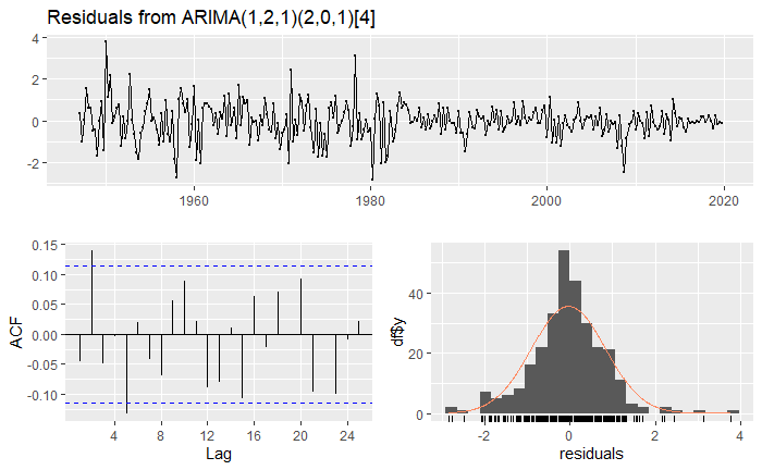
The Ljung-Box test and the plot show that there is autocorrelation in the residuals. We can reject the null-hypothesis that there is no autocorrelation at the 1% level. This illustrates that, while auto.arima() is efficient, it is always a good idea to review the model it selects.
auto.arima() contains a lot of flexibility. If one knows the value of \(d\), it can be passed to the function. Maximum and starting values for \(p,q,\) and \(d\) can be specified in the seasonal- and non-seasonal cases. If one would like to restrict themselves to a non-seasonal model, or use a different test, these can also be done. Some of these features are demonstrated below. The method for testing unit roots can also be specified. See ?auto.arima or the package documentation for more.
# Auto-estimate y, specifying:
## non-seasonal
## Using Augmented Dickey-Fuller rather than KPSS
## d=1
## p starts at 1 and does not exceed 4
# no drift
lgdp_ns <- auto.arima(y,
                      seasonal = F,
                      test = "adf",
                      start.p = 1,
                      max.p = 4,
                      allowdrift = F)
#An ARIMA(3,1,0) was specified
lgdp_ns
The forecast package also contains the ability to simulate ARIMA data
given an ARIMA model. Note that the input here should come from either
forecast::auto.arima() or forecast::Arima(), rather than
stats::arima().
#Simulate data using a non-seasonal ARIMA()
arima_222 <- Arima(y, c(2,2,2))
sim_arima <- forecast:::simulate.Arima(arima_222)
tail(sim_arima, 20)