Spatial Joins
Spatial joins are crucial for merging different types of data in geospatial analysis. For example, if you want to know how many libraries (points) are in a city, county, or state (polygon). This skill allows you to take data from different types of spatial data (vector data like points, lines, and polygons, and raster data (with a little more work)) sets and merge them together using unique identifiers.
Joins are typically interesections of objects, but can be expressed in different ways. These include: equals, covers, covered by, within, touches, near, crosses, and more. These are all functions within the sf function in R or the geopandas package in Python. For more on the different types of intersections in 2D projections, see the Wikipedia page on spatial relations.
Keep in Mind
- Geospatial packages in R and Python tend to have a large number of complex dependencies, which can make installing them painful. Best practice is to install geospatial packages in a new virtual environment.
- When it comes to the package we are using in R for the US boundaries, it is much easier to install via the devtools. This will save you the trouble of getting errors when installing the data packages for the boundaries. Otherwise, your mileage may vary. When I installed USAboundariesData via USAboundaries, I received errors.
devtools::install_github("ropensci/USAboundaries")
devtools::install_github("ropensci/USAboundariesData")
- Note: Even with the R installation via devtools, you may be prompted to install the “USAboundariesData” package and need to restart your session.
Implementations
Python
The geopandas package is the easiest way to start doing geo-spatial analysis in Python. This example of a spatial merge closely follows one from the documentation for geopandas.
# Geospatial packages tend to have many elaborate dependencies. The quickest
# way to get going is to use a clean virtual environment and then
# 'conda install geopandas' followed by
# 'conda install -c conda-forge descartes'
# descartes is what allows geopandas to plot data.

import geopandas as gpd

# Grab a world map
world = gpd.read_file(gpd.datasets.get_path('naturalearth_lowres'))

# Plot the map of the world
world.plot()

# Grab data on cities
cities = gpd.read_file(gpd.datasets.get_path('naturalearth_cities'))

# We can plot the cities too - but they're just dots of lat/lon without any
# context for now
cities.plot()

# The data don't actually need to be combined to be viewed on a map as long as
# they are using the same 'crs', or coordinate reference system.
# Force cities and world to share crs:
cities = cities.to_crs(world.crs)

# Combine them on a plot:
base = world.plot(color='white', edgecolor='black')
cities.plot(ax=base, marker='o', color='red', markersize=5)

# We want to perform a spatial merge, but there are many kinds in 2D
# projections, including withins, touches, crosses, and overlaps. We want to
# use an intersects spatial join - ie we want to combine each city (a lat/lon
# point) with the shapes of countries and determine which city goes in which
# country (even if it's on the boundary). We use the 'sjoin' function:

cities_with_country = gpd.sjoin(cities, world, how="inner", op='intersects')

cities_with_country.head()
#  name_left                   geometry    pop_est     continent  \
#  Vatican City  POINT (12.45339 41.90328)   62137802    Europe
#    San Marino  POINT (12.44177 43.93610)   62137802    Europe
#          Rome  POINT (12.48131 41.89790)   62137802    Europe
#         Vaduz   POINT (9.51667 47.13372)    8754413    Europe
#        Vienna  POINT (16.36469 48.20196)    8754413    Europe
#  name_right iso_a3  gdp_md_est
#       Italy    ITA   2221000.0
#       Italy    ITA   2221000.0
#       Italy    ITA   2221000.0
#     Austria    AUT    416600.0
#     Austria    AUT    416600.0
R
Acknowledgments to Ryan A. Peek for his guide that I am reimagining for LOST.
We will need a few packages to do our analysis. If you need to install any packages, do so with install.packages(‘name_of_package’), then load it if necessary.
library(sf)
library(dplyr)
library(viridis)
library(ggplot2)
library(USAboundaries)
library(GSODR)
-
We will work with polygon data from the USA boundaries initially, then move on to climate data point data via the Global Surface Summary of the Day (gsodr) package and join them together.
-
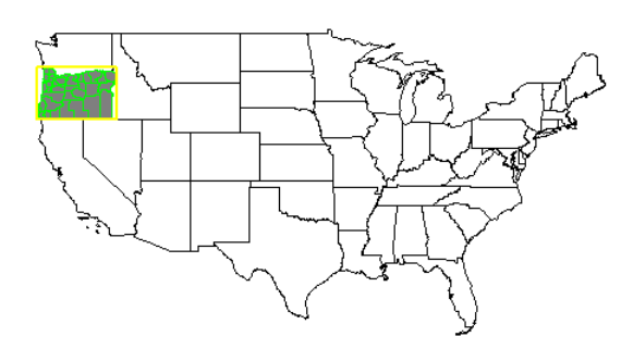
We start with the boundaries of the United States to get desirable polygons to work with for our analysis. To pay homage to the states of my alma maters, we will do some analysis with Oregon, Ohio, and Michigan.
#Selecting the United States Boundaries, but omitting Alaska, Hawaii, and Puerto Rico for it to be scaled better

usa <- us_boundaries(type="state", resolution = "low") %>%
  filter(!state_abbr %in% c("PR", "AK", "HI"))

#Ohio with high resolution
oh <- USAboundaries::us_states(resolution = "high", states = "OH")

#Oregon with high resolution
or <- USAboundaries::us_states(resolution = "high", states = "OR")

#Michigan with high resolution
mi <- USAboundaries::us_states(resolution = "high", states = "MI")

#Insets for the identified states

#Oregon
or_box <- st_make_grid(or, n = 1)

#Ohio
oh_box <- st_make_grid(oh, n = 1)

#Michigan
mi_box <- st_make_grid(mi, n = 1)

#We can also include the counties boundaries within the state too!

#Oregon
or_co <- USAboundaries::us_counties(resolution = "high", states = "OR")

#Ohio
oh_co <- USAboundaries::us_counties(resolution = "high", states = "OH")

#Michigan

mi_co <- USAboundaries::us_counties(resolution = "high", states = "MI")
Now we can plot it out.
Oregon highlighted
plot(usa$geometry)
plot(or$geometry, add=T, col="gray50", border="black")
plot(or_co$geometry, add=T, border="green", col=NA)
plot(or_box, add=T, border="yellow", col=NA, lwd=2)
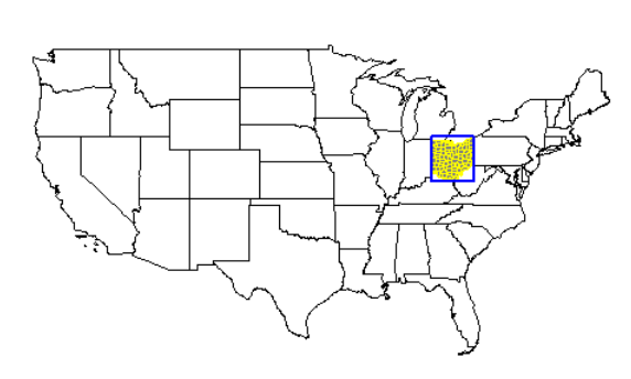
Ohio highlighted
plot(usa$geometry)
plot(oh$geometry, add=T, col="gray50", border="black")
plot(oh_co$geometry, add=T, border="yellow", col=NA)
plot(oh_box, add=T, border="blue", col=NA, lwd=2)
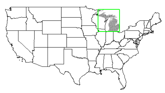
Michigan highlighted
plot(usa$geometry)
plot(mi$geometry, add=T, col="gray50", border="black")
plot(mi_co$geometry, add=T, border="gray", col=NA)
plot(mi_box, add=T, border="green", col=NA, lwd=2)
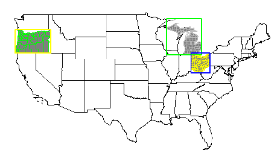
All three highlighted at once.
plot(usa$geometry)
plot(mi$geometry, add=T, col="gray50", border="black")
plot(mi_co$geometry, add=T, border="gray", col=NA)
plot(mi_box, add=T, border="green", col=NA, lwd=2)
plot(oh$geometry, add=T, col="gray50", border="black")
plot(oh_co$geometry, add=T, border="yellow", col=NA)
plot(oh_box, add=T, border="blue", col=NA, lwd=2)
plot(or$geometry, add=T, col="gray50", border="black")
plot(or_co$geometry, add=T, border="green", col=NA)
plot(or_box, add=T, border="yellow", col=NA, lwd=2)
Now that there are polygons established and identified, we can add in some point data to join to our currently existing polygon data and do some analysis with it. To do this we will use the Global Surface Summary of the Day (gsodr) package for climate data.
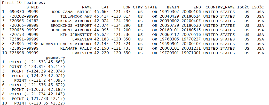
We will take the metadata from the GSODR package via ‘isd_history’, make it spatial data, then filter out only those observations in our candidate states of Oregon, Ohio, and Michigan.
load(system.file("extdata", "isd_history.rda", package = "GSODR"))

#We want this to be spatial data
isd_history <- as.data.frame(isd_history) %>%
  st_as_sf(coords=c("LON","LAT"), crs=4326, remove=FALSE)

#There are many observations, so we want to narrow it to our three candidate states
isd_history_or <- dplyr::filter(isd_history, CTRY=="US", STATE=="OR")
isd_history_oh <- dplyr::filter(isd_history, CTRY=="US", STATE=="OH")
isd_history_mi <- dplyr::filter(isd_history, CTRY=="US", STATE=="MI")
This filtering should take you from around 26,700 observation sites around the world to approximately 200 in Michigan, 85 in Ohio, and 100 in Oregon. These numbers may vary based on when you independently do your analysis.
Let’s see these stations plotted in each state individually:
Note: the codes in the ‘border’ and ‘bg’ identifiers are from the viridis package. You can get some awesome color scales using that package. You can also use standard names.
Oregon
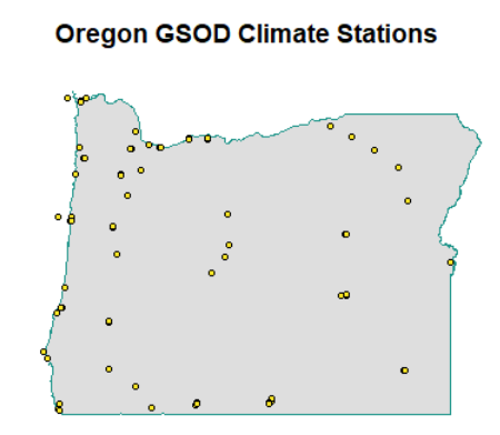
plot(isd_history_or$geometry, cex=0.5)
plot(or$geometry, col=alpha("gray", 0.5), border="#1F968BFF", lwd=1.5, add=TRUE)
plot(isd_history_or$geometry, add=T, pch=21, bg="#FDE725FF", cex=0.7, col="black")
title("Oregon GSOD Climate Stations")
Ohio
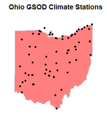
plot(isd_history_oh$geometry, cex=0.5)
plot(oh$geometry, col=alpha("red", 0.5), border="gray", lwd=1.5, add=TRUE)
plot(isd_history_oh$geometry, add=T, pch=21, bg="black", cex=0.7, col="black")
title("Ohio GSOD Climate Stations")
Michigan
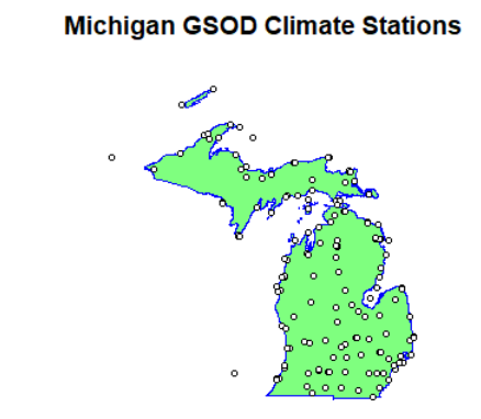
plot(isd_history_mi$geometry, cex=0.5)
plot(mi$geometry, col=alpha("green", 0.5), border="blue", lwd=1.5, add=TRUE)
plot(isd_history_mi$geometry, add=T, pch=21, bg="white", cex=0.7, col="black")
title("Michigan GSOD Climate Stations")
Now, for the magic:
We are going to start with selecting polygons from points. This is not necessarily merging the data together, but using a spatial join to filter out polygons (counties, states, etc.) from points (climate data stations)
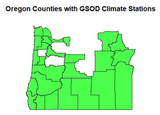
We will start by selecting the Oregon counties that have climate data stations within their boundaries:
or_co_isd_poly <- or_co[isd_history, ]
plot(or_co_isd_poly$geometry, col=alpha("green",0.7))
title("Oregon Counties with GSOD Climate Stations")
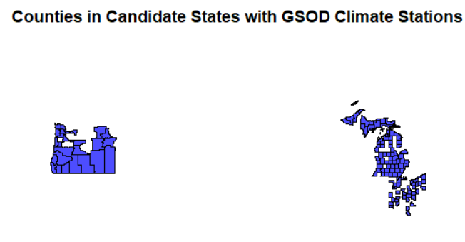
Now for all of our three candidate states:
cand_co <- USAboundaries::us_counties(resolution = "high", states = c("OR", "OH", "MI"))
cand_co_isd_poly <- cand_co[isd_history, ]
plot(cand_co_isd_poly$geometry, col=alpha("blue",0.7))
title("Counties in Candidate States with GSOD Climate Stations")
We see how we can filter out polygons from attributes or intersecting relationships with points, but what if we want to merge data from the points into the polygon or vice versa?
We will use the data set for Oregon for the join example.
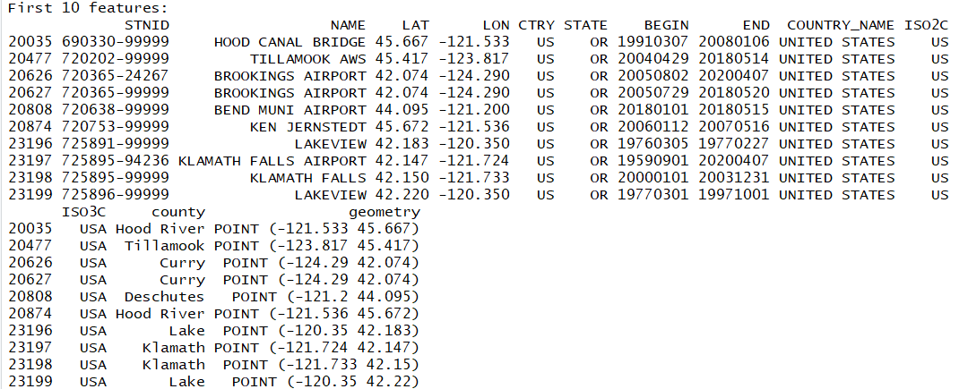
Notice in our point dataset that there are no county names. Only station/city names.
Let us join the county polygons with the climate station points and add the county names to the station data. We do this using the st_join function, which comes from the sf package.
isd_or_co_pts <- st_join(isd_history, left = FALSE, or_co["name"])

#Rename the county name variable county instead of name, since we already have NAME for the station location

colnames(isd_or_co_pts)[which(names(isd_or_co_pts) == "name")] <- "county"

plot(isd_or_co_pts$geometry, pch=21, cex=0.7, col="black", bg="orange")
plot(or_co$geometry, border="gray", col=NA, add=T)
You now have successfully joined the county name data into your new point data set! Those points in the plot now contain the county information for data analysis purposes.
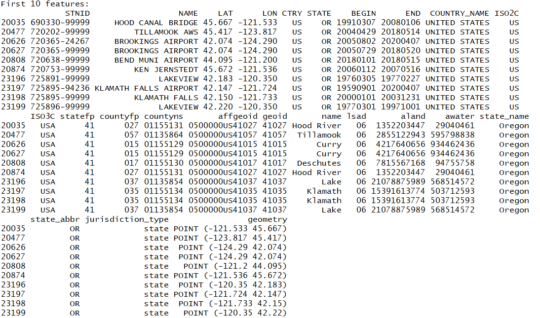
You can join in any attribute you would like, or by leaving it as:
isd_or_co_pts <- st_join(isd_history, left = FALSE, or_co)
You add all attributes from the polygon into the point data frame!
Also note that st_join is the default function that joins any type of intersection. You can be more precise our particular about your conditions with the other spatial joins:
st_within only joins elements that are completely within the defined area
st_equal only joins elements that are spatially equal. Meaning that A is within B and B is within A.
You can use these to pare down your selections and joins to specific relationships.
Good luck with your geospatial analysis!